3D Hydrodynamics - Taylor Green Vortex#
Problem setup#
The Taylor-Green vortex is a well-known analytical solution used to validate numerical methods for solving the Navier-Stokes equations. It describes the decay of a vortex in a periodic domain and can be characterized by the following initial conditions:
This can be setup through the pre-defined cased built into the solver but for this case it will be shown through the custom initial condition method.
Adding the following in pre_proc/init_modes/init_hydro.py is equivalent to defining the equations specified previously:
X, Y, Z = ncp.meshgrid( ncp.linspace(0,2*ncp.pi,para.Nx),
                        ncp.linspace(0,2*ncp.pi,para.Nz),
                        ncp.linspace(0,2*ncp.pi,para.Nz),
                        indexing = 'ij')

Vx =   ncp.sin(X) * ncp.cos(Y) * ncp.cos(Z)
Vy = - ncp.cos(X) * ncp.sin(Y) * ncp.cos(Z)
Vz =   ncp.zeros((para.Nx, para.Ny, para.Nz))

from TARANG.lib.global_fns.spectral_setup import forward_transform

Vkx = forward_transform(Vx, Vkx)
Vky = forward_transform(Vy, Vky)
Vkz = forward_transform(Vz, Vkz)
Specifying parameters#
para.py defines all the key parameters needed to run a simulation. It controls aspects like computational settings (CPU/GPU), grid resolution, numerical schemes, and data output frequency.
device = 'CPU'                     # 'CPU' or 'GPU' depending on device

device_rank = 0                    # Rank of GPU device if 'GPU' is selected

kind = 'HYDRO'                     # Type of simulation (e.g., 'HYDRO' for hydrodynamics)

INPUT_SET_CASE = True              # Whether to use a predefined case or custom initial conditions
input_case = 'custom'              # Name of the input case if INPUT_SET_CASE is True

dimension = 3                      # Number of spatial dimensions

Nx = 64                            # Number of grid points in the x, y or z direction
Ny = 64
Nz = 64

BOX_SIZE_DEFAULT = True            # Whether to use the default box size

nu = 2E-2                          # Kinematic viscosity

FORCING_ENABLED = False            # Whether external forcing is enabled

time_scheme = 'RK4'                # Time integration scheme (e.g., 'RK4' for Runge-Kutta 4th order)

t_initial = 0                      # Initial time
t_final = 0.1                      # Final time
dt = 1E-3                          # Time step size

FIXED_DT = True                    # Whether to use a fixed time step size

PRINT_PARAMETERS = True            # Whether to print simulation parameters

iter_field_save_start = t_initial  # Iteration to start saving field data
iter_field_save_inter = 10         # Interval between saving field data

iter_glob_energy_print_start = t_initial # Iteration to start printing global energy
iter_glob_energy_print_inter = 1         # Interval between printing global energy

iter_ekTk_save_start = t_initial   # Iteration to start saving kinetic and thermal energy
iter_ekTk_save_inter = 100         # Interval between saving kinetic and thermal energy

iter_modes_save_start = t_initial  # Iteration to start saving mode data
iter_modes_save_inter = 1000       # Interval between saving mode data
Running the code#
To execute the solver, simply run the tarang_cli.py script:
python3 tarangc_cli.py
Note: All commands have to be run from the root directory of the solver bundle i.e. from the same directory as para.py or tarang_cli.py.
This will produce an output similar to the following:
TARANG

Running SEQUENTIAL SOLVER on CPU at rank 0 with PID 23986
Output path = path/to/output

Dimension = 3
Grid resolution = [64, 64, 64]
Box size = [6.283185307179586, 6.283185307179586, 6.283185307179586]

Time scheme = RK4
t_initial = 0
t_final = 0.1
dt = 0.001

Modes probe = [(1, 0)]


Problem kind is HYDRO

Active viscous dissipation = ['(0.02)k^{2}']

No external forcing: Decaying simulation


t dt Eu div_u eps_u
0 0.001 0.1269221305847168 0.0063320332538278805 0.015459800502509778
0.001 0.001 0.1269066748347258 0.00620342397542081 0.015454026933944532
.
.
.
0.099 0.001 0.12541488571622883 0.0040294741577690425 0.015165272911464895
0.1 0.001 0.12539981920696336 0.004028990649881165 0.015163389575288982

Compute time = 17.182244062423706

Time per step = 0.17182244062423707
Output Structure#
If the same parameters were used, the output directory will contain the following structure:
output/
├── ekTk.h5                # Energy spectrum data
├── fields/                # Solution snapshots
│   ├── Soln_0.000000.h5
│   ├── Soln_0.010000.h5
│   ├── ...
│   └── Soln_0.100000.h5
├── glob.h5                # Global diagnostics data like energy, dissipation rate
├── modes.h5               # Mode-specific time evolution
├── para.py                # Parameter file
├── paraIO.py              # Input/output configuration
├── t_dt.h5                # Time step evolution
└── t_field_save.h5        # Field saving time data
Soln_X.XXXXXX.h5 (Field Snapshots)#
Captures the state of the velocity field at different time steps during the simulation.
Soln_X.XXXXXX.h5
├Vkx        [(r: float64, i: float64): 64 × 64 × 33]    # X-component of the Velocity Fourier field
├Vky        [(r: float64, i: float64): 64 × 64 × 33]    # Y-component of the Velocity Fourier field
└Vkz        [(r: float64, i: float64): 64 × 64 × 33]    # Z-component of the Velocity Fourier field
ekTk.h5 (Energy Spectrum Data)#
Contains the evolution of kinetic energy (ek) and transfer functions (Tk) over time.
ekTk.h5
├ Tk    [float64: 2 × 57 × 3]    # Transfer function at different time steps
├ ek    [float64: 2 × 57 × 3]    # Energy spectrum values
├ k     [float64: 57]            # Wavenumber array
└ t     [float64: 2]             # Time instances corresponding to stored values
glob.h5 (Global Diagnostics)#
Stores integral quantities describing the overall evolution of the flow.
glob.h5
├ Eu                [float64: 101] # Total kinetic energy over time
├ Eu_dissipation    [float64: 101] # Energy dissipation rate
├ div_v             [float64: 101] # Divergence of velocity field
└ t                 [float64: 101] # Time array
modes.h5 (Mode Evolution)#
Tracks the evolution of selected Fourier modes over time.
modes.h5
├ modes_Vx     [(r: float64, i: float64): 2 × 1 × 33]  # X-component mode values (real & imaginary)
├ modes_Vy     [(r: float64, i: float64): 2 × 1 × 33]  # Y-component mode values (real & imaginary)
├ modes_Vz     [(r: float64, i: float64): 2 × 1 × 33]  # Z-component mode values (real & imaginary)
└ t            [float64: 2]                            # Time instances
t_dt.h5 (Time Step Evolution)#
Stores the time step (dt) used during the simulation.
t_dt.h5
├ dt      [float64: 100] # Time step values at different iterations
└ t       [float64: 100] # Corresponding time array
t_field_save.h5 (Field Saving Times)#
Records the time instances at which field snapshots were saved.
t_field_save.h5
└ t       [float64: 11]  # Time steps when solution snapshots were stored
Post-processing#
To generate post-processing plots, run the post_proc/post_proc.py script while specifying the required plot type in command line arguments:
python3 post_proc/post_proc.py '<output_plot_dir>' '<t_initial> <t_final>' spectrum energy flux field
'<output_plot_dir>': The directory where the generated plots will be saved.'<t_initial> <t_final>': The initial and final time for averaged plots. If both are equal plot will be made for a single frame.spectrum: Generates a spectrum plot.energy: Generates an energy plot.flux: Generates a flux plot.field: Generates a field quiver plot.
Note: Do not forget the quotation marks for output directory and the time entries.
Running this script should give the following plots displayed and stored in output/plots folder for $T = 0.1$:
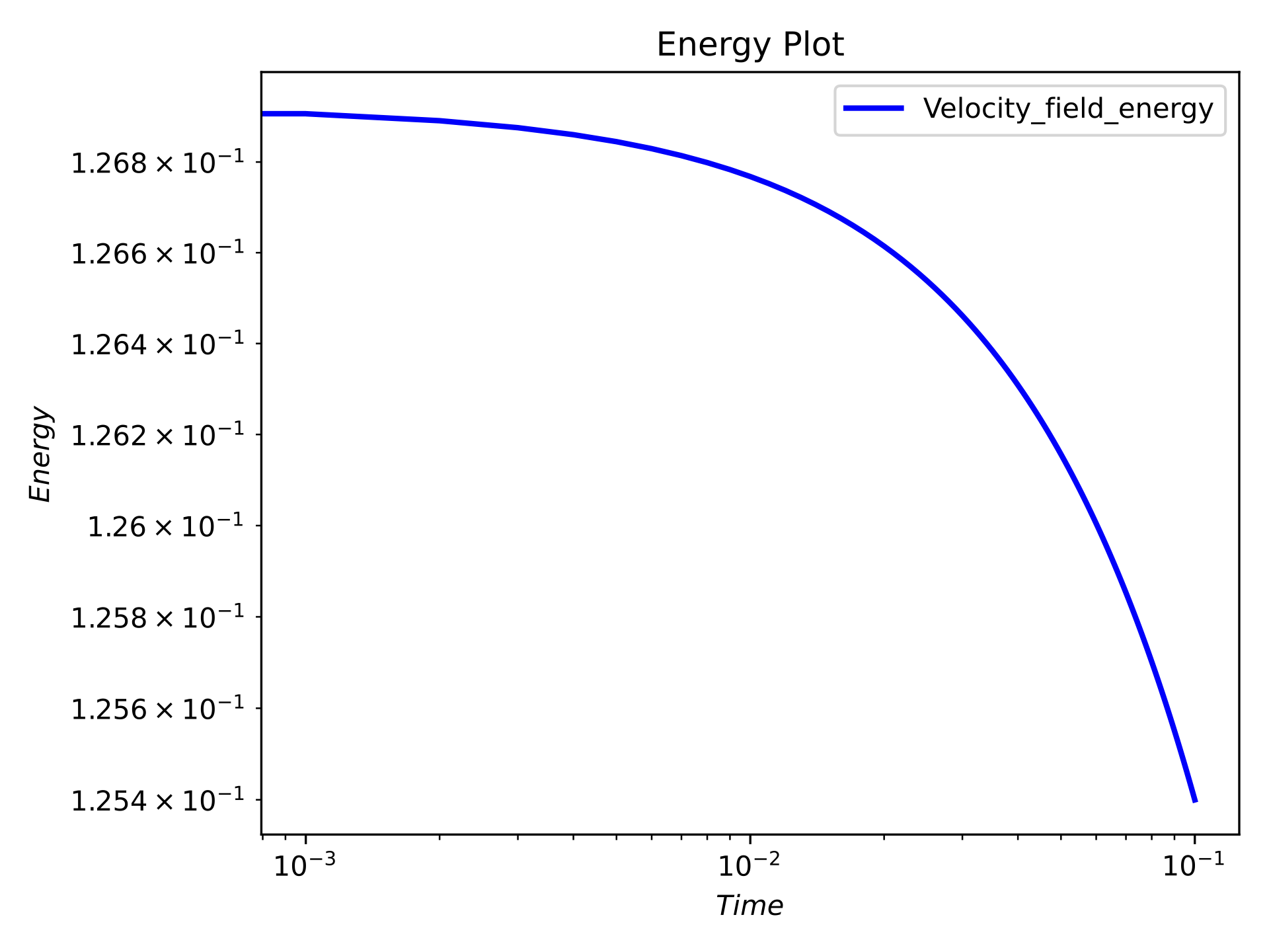
Time series energy plot#
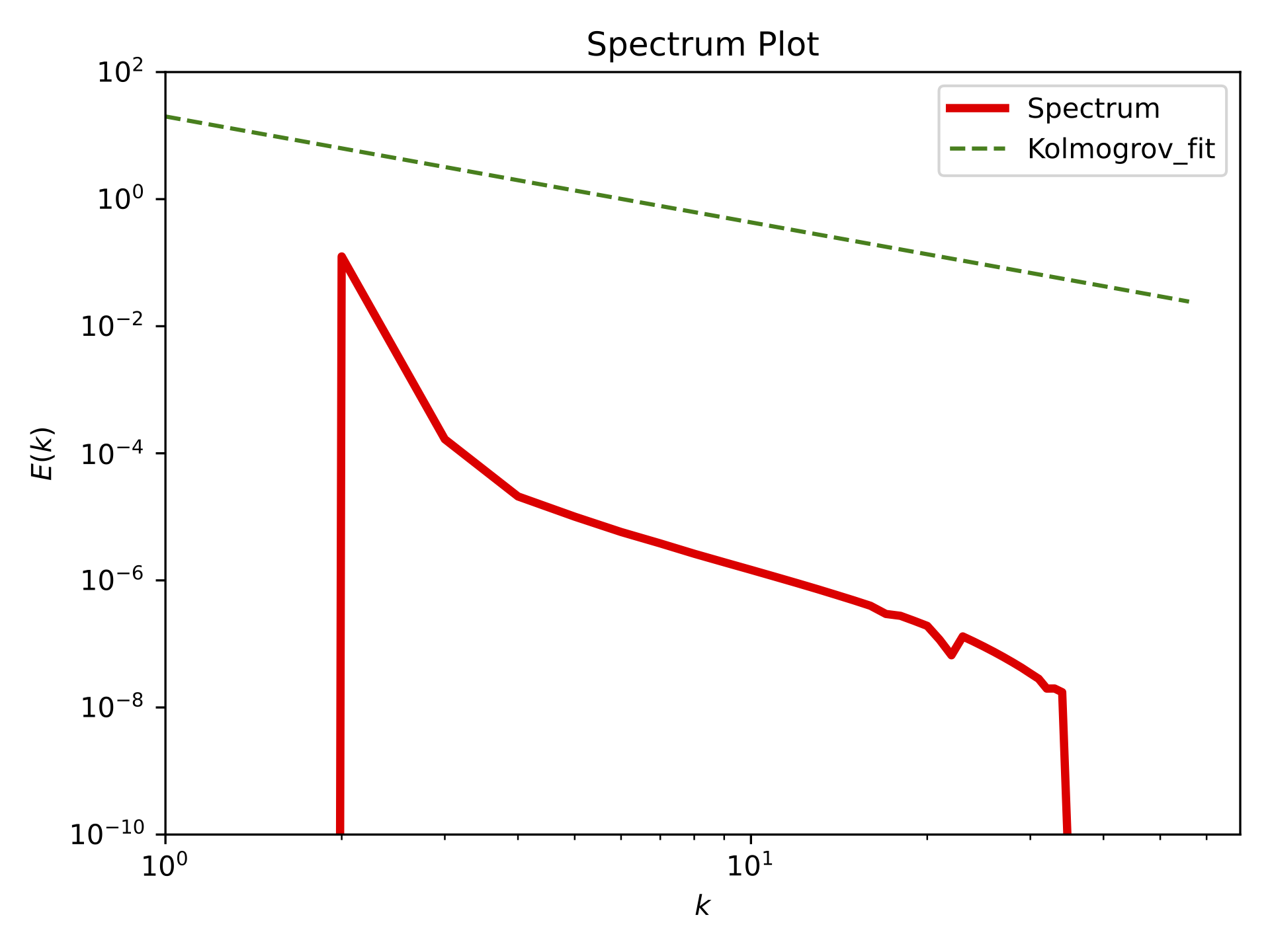
Spectrum plot at T=0.1#
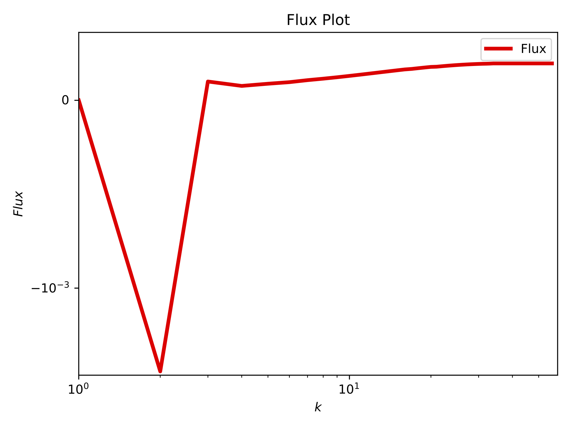
Flux plot at T=0.1#
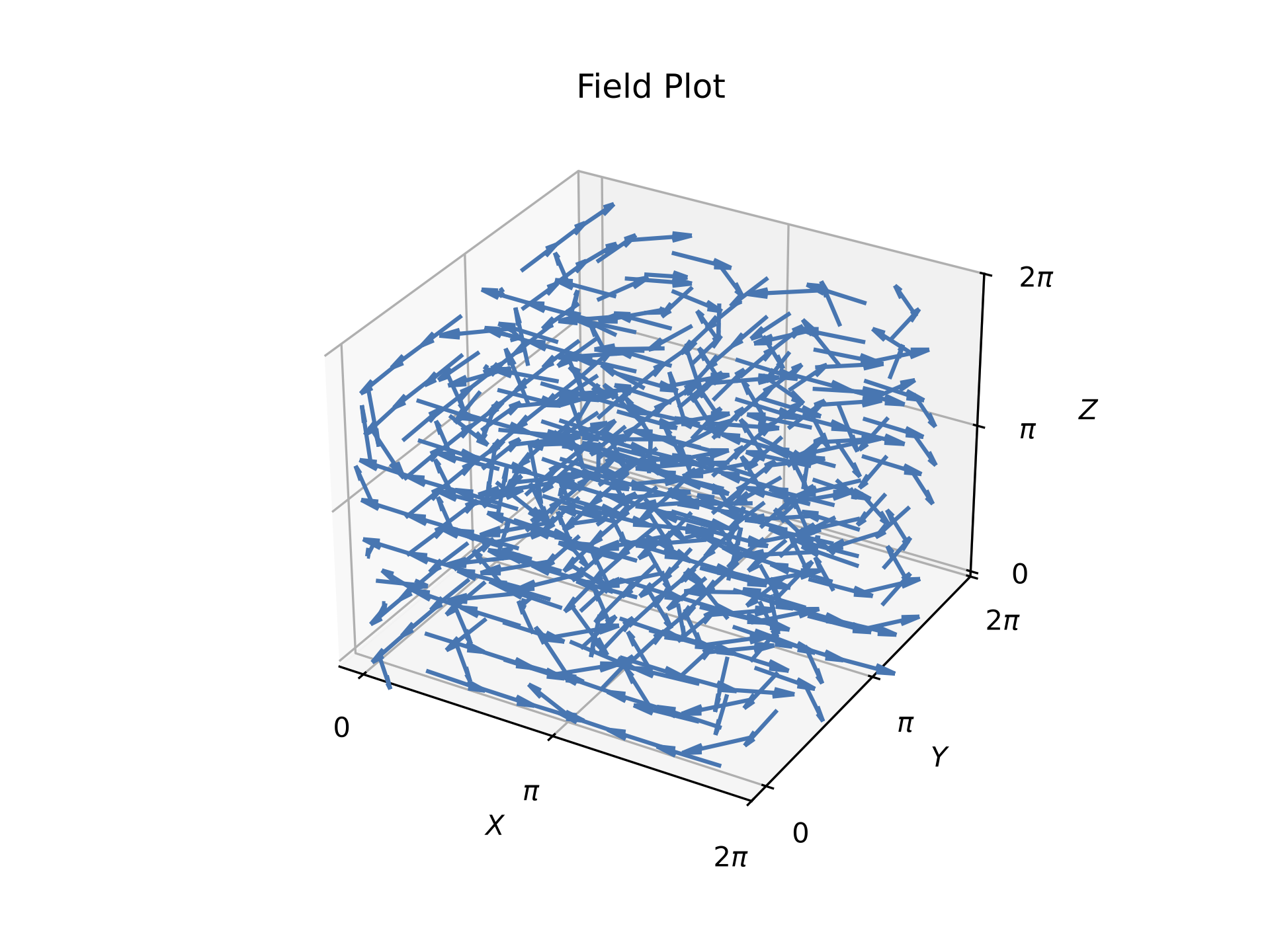
Field snapshot at T=0.1#